The BedloadWeb project
BedloadWeb results from a collaboration between INRAE and l'Office Francais de la Biodiversite


The english version of this website was funded by the AlpineSpace European project 'HyMoCARES'

Welcome on bedloadWeb
BedloadWeb is the online version of the program BedloadR.R which objectives is to make it easy visualization data from the literature, and to offer assistance in calculating the sediment transport associated with a flow section. It aims to be a collaborative platform to encourage exchanges between researchers and practitioners, but also, to be educational for students

Update 01/03/2023
Shear stress correction
In the last version, the "Shear stress correction" option was checked by default when constructing a new section (see: Model > Sediment Transport > Calculation). Following user request, this option is now unchecked by default.

Update 01/03/2023
Makeover
The menu has been redesigned for better program ergonomics. The basic functions have not changed, but are just accessible a little differently. In particular, the database tab has been moved to the end of the menu.
Local Backup
Due to the strong evolution of the program, it is no longer possible to save the data on your PC in txt format. You can still save locally in ZIP format, but compared to the txt format, this requires an account. If you want to read old txt backups, you can ask for help from one of the site contacts.
Data management
A big difference with the previous version is that you can now manage your data (granulo, section) independently from modeling considerations
Import several sections
As a consequence of the previous point, it is now possible to import several sections from a txt file with one click
New Tools
New tools are available. You can quickly draw a sedimentary profile (bedload transport along the longitudinal profile) for a given flow Q. You can also investigate the effects of natural data variability on sediment transport calculations.
Equations
A modification concerns the calculation of tm* in the Recking Equation 2013 (see details in table 'Connexion > your settings')

Update 01/05/2021
Debug
Several bugs have been reported to us and have been corrected, especially in saving granulos and photos. Any new version is likely to contain bugs; do not hesitate to let us know (contact on the 'help' page).
Zip
It is now possible to save your project on your PC in a zip file. Unlike the existing txt save, this option allows you to save the entire project, including the photos. MENU: Your Project> Local Backup> ‘Zip’ option
Archiving
The project management menu now gives you the option to archive your unused files
Coming next
Follow the news, the code being constantly evolving. Coming soon: ucertainties calculation, GIS management, provision of the BedloadR code….
Quick start
The "database" and "Project" parts are independent and can be approached separately. The database does not allow any calculations, but just to visualize bedload measurements and the models. The Project part allows you to make calculations.
Participative
All information likely to improve the platform are welcome (photos, new data, comments, questions ...). This is especially true during the 'break-in' phase of the site. Any anomalies can be quickly corrected provided they are reported to us
New equations can also be added to the tools already available.
Condition of use
BedloadWeb is free to access. A reference (or web link) to the original publication is always given and must be recalled whenever a dataset is used. The authors would also appreciate the fact that the BedloadWeb platform is cited when it is used.
Training
BedloadR is used as a support for training in sediment transport and river geomorphology. A basic session, in the form of a mini-project, explains how to carry out a sediment budget (explanation of basic concepts, collection of the necessary data, study of uncertainties, etc.). An advanced session is for people who know the R language and want to integrate their own module into BedloadR. These sessions can be personalized, to take into account the level of knowledge of the public concerned. A quote can be sent to you on request by email.
Having an account is not mandatory to use the following calculation tabs
However, an account is mandatory if you want to save or share your data.
The server only accepts files encoded in UTF8. But locally (on your PC with BedloadR.R), the backups will be UTF8 except for certain files where special characters have been entered (é..), which will be saved with the PC's encoding system (ANSI, etc.). . Importing such a ZIP project to the server will cause a crash. The solution is to not enter any special characters at all, or else convert to UTF8 with this option:
CAUTION: Do not use this UTF8 conversion if the ZIP project is to be shared locally (with BedloadR.R in a PC) as there will be issues displaying special characters ("é" becomes "Ã@"). It will be the same if you open with BedloadR.R a project created with BedloadWeb.
Save the project in a zip file
Create backup
Import a zip backup
This option allows you to save your project locally, in a zip file. Unlike the previous txt option (which does not exist anymore), the project must first have been saved to an account. The advantage of this solution is that it saves the entire project, including photos. Opening a zip project on your account cannot be done under the same name as an existing project (if this is the case, you will have to propose a new name in the box provided for this purpose).
Create an account
Email is not mandatory at this stage. But be aware that, for reasons of confidentiality, in the absence of a valid email associated with the account it will no longer be possible to access the account in case of forgotten password.
This code will be asked if you want to exchange folders with another user; it can be defined later from the 'Manage Account' tab
Selected project:
Warning: will only be saved in the project what has already been saved elsewhere in the different tabs
Project management:
By creating an account you can save your projects on the server, including photos and project description
Enter the name of the project:
Available projects:
You have two options to transfer a project to another user: OPTION1 you export the project locally on your PC and you transfer the resulting text file, which can be open by the other user (warning: this option does not take into account the photos and the text 'project description'). OPTION2, you and your contact have a user account and you can use the function below: for this you need to know its identifier (pay attention to lower / upper case), and its share code (different from its password!)
Delete a project from this list to make it reappear in the list of available projects
You must re-enter your password to access account changes
Change password:
Change the mail adress:
Files sharing code
This series of tools assists you in a sediment budget study. It consists of several tabs each of which represents an essential step for a serious study. The tabs are presented in a logical sequence, each producing useful data for the following: - the 'Granulometry' tab allows you to define the particle size of the sediments - the 'Section' tab allows you to define (topography) and dress ( roughness ..) the flow section - the 'hydraulic' tab is used to calculate the main hydraulics parameters for the normal uniform regime - the 'solid transport' tab calculates the fluxes for the granulometry, the section and hydraulics previously defined 5) the 'hydrology' tab permts to defien an hydrology and to compute the associated sediment budget
You can save your entry (except photos) in text format on your PC, or create an account (the backup on the server gives access to a project management menu, and allows you to save photos).
Here you can set some calculation options for the project
Project:
Preselect the equations to display by default
In case of single choice:
In case of multiple choice:
In the previous version of the program, a formulation tm*=f(S, D84/D50) was used for the riffle-pools, alternate bars and wandering morphologies, whereas the formulation tm*=1.5S^0.75 was used for the others morphologies.
A difficulty came from the fact that not everyone has the same appreciation of the morphology (limit between braiding, riffle-pool and alternate bars, etc.), and moreover the formulation tm*=f(S, D84/D50) is not valid for steep slopes >3%.
In this new version of the program the calculation is tm*=1.5S^0.75 by default for all morphologies. To find the previous calculation, this option must be validated.
This page allows you to create a database containing the grain size distributions of your project
This database will then be accessible from the other pages of the program
Input options:
You can enter several samples to define a grain size curve (and manage the samples with the menu on the right).
You can enter the number of pebbles measured in each diameter class (Wolman method) in the next table. you can also reproduce a realistic curve from the D50 (model deduced from the analysis of more than a hundred curves measured in the field).
More information on the model in Recking, A. (2013), An analysis of non-linearity effects on bedload prediction, Journal of Geophysical Research - Earth Surface, 118, 1-18, doi: 10.1002/jgrf.20090
Input format
Here you must enter the geometry of your sections
This data will then be available from the other pages of the program
Easy built with trapezes
Use this tool to quickly build a section composed from trapezes
Import a file
Be careful: new format!
Here you can import in a single text file all the sections of your project.
The data must be arranged in 2 columns separated by a semicolon, following a strict format, to be repeated without interruption for each section (data may be missing, but the number of lines must be respected with "SEC" at the start and ";" on each line): Example file
LINE1: [SEC; section name] (SEC allows the program to locate the beginning of each new section)
LIGNE2: [longitude; latitude]
LINE3: [PK; Reach] (default set to 1 for Reach)
LIGNE4: [slope;date]
LINE 5 and following: Values [X; Z] describing the cross section. Left Bank to Right Bank by convention but it doesn't matter as long as the sections are all described in the same way. Check data quality, for example avoiding non-numeric characters or missing values
The slope must be entered in m/m (ex S = 1% = 0.01 m/m). This is a very important parameter and must be filled in carefully. It must be defined for the calculation section over a distance at least equal to 10 times the width of the main channel. In the majority of cases it will be the slope of the stream bed (measured of the water line at low flow). On the other hand, for very low slopes (S < 0.001m/m) the geometric slope will replaced by the flow slope, and it will be necessary to use the latter (to be measured in flood, or to simulate with 1D model, or search in the archives).
Slope (m/m):
Manual entry:
Whatever the input mode (keystone, file import) the data is copied into this table from where they can be modified manually
Modelling with trapezes
Enter dimensions (m)
Bottom level (m)
BedloadR calculates the hydraulics of each section assuming normal flow (water depth not influenced downstream)
If your sections are influenced downstream (water height controled by a dam for instance) you can enter here Q(H,S) calibration laws resulting from measurements or numerical modeling
These laws can later, for each section, be called in the "Hydraulic" section, to build the model
Default slope [m/m]:
In case of problem when entering the decimals, edit the cell by double clicking on it
This page allows you to create a database containing the hydrographs Q(t) of your project
This database will then be accessible from the other pages of the program
Hydrology input
Build a hydrograph
This tool allows you to quickly construct a theoretical triangular hydrograph FOR THE SECTION WHICH IS OPENED IN THE MODELLING TAB. parameters will be automatically proposed for this section. The values are given by default, and can be modified
Import a file
Import your time (unit of your choice) / flow (m3 / S) data from text files. The data must be arranged in 2 columns separated by tabs and containing titles (eg T, Q. Avoid special caracters!). Describe the values by increasing T. Check the quality of the data, for example by avoiding non-numeric characters or missing values
The text file should have two columns separated by tabulation
Colomn1 'FND': Frequency of non-exceedance x 100. WARNING: data must be entered in decreasing order!
Colonne2 'Q': associated discharge m3/s
Recall
T=1/FD
FD=1-FND
FD(j/an)=(1-FND)*365
Unites
A hydrograph is discretized at the indicated time step. For example, a triangular hydrograph of 1200 minutes will generate a file of 1200 points, even if you defined it with 3 points only. This can be problematic with large hydrographs (for example 1 month hydrograph with a minute time step generates a file of more than 40,000 values, which will complicate certain calculations such as MonteCarlo analyzes). This function makes it possible to reduce the size of the hydrograph by converting the sampling step (s-> min, min-> h, etc.). If you save the hydrograph and the project the change will be final. It is therefore advisable to replicate the hydrograph and make the change on the copy.
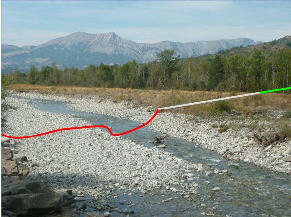
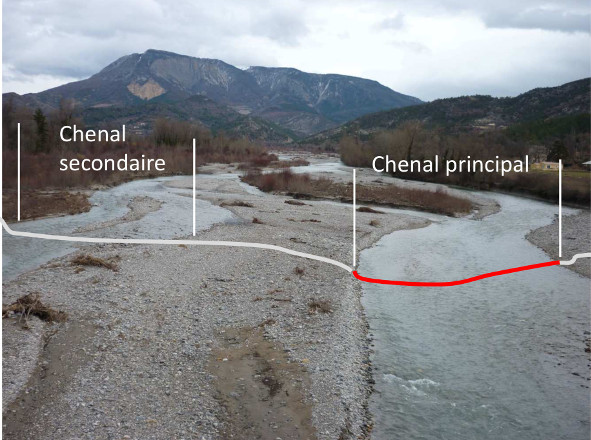
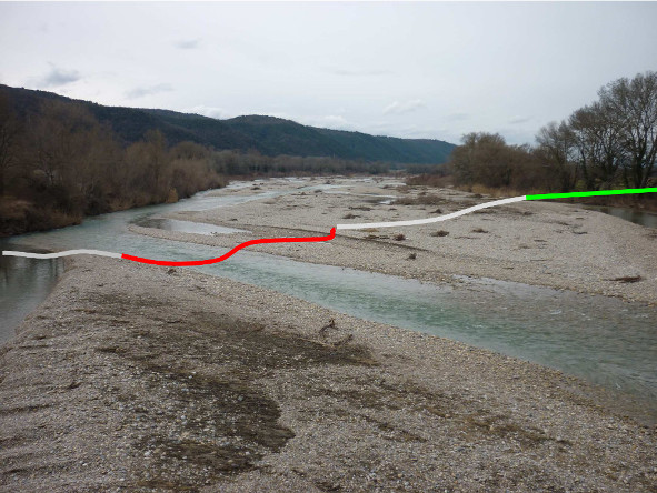
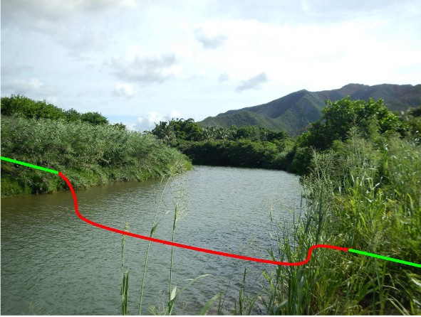
Here you must specify what makes up each section (limits of the main channel, presence of vegetation, etc.)
Pay attention to this step, which will have a major impact on your results (the following tabs will only repeat this data to display the associated hydraulics and solid transport).
Main channel
The main channel (usuallly a few tens of meter) is the part of bed that transfers the current floods, it must be differentiated from the flood plain (often > 100m).
Its definition is very important because it directly impacts the calculation of the hydraulic radius R used in the calculation of bedload transport
As R = wetted area / wetted perimeter, a too large width will produce very low or even decreasing R values if calculated for very shallow flow over the flood plain
To avoid this, the calculation is limited to the main channel to be defined by the user (in general a few tens of meters).
You can test the effect of different widths by comparing the R(H) curves in the HYDRAULICS page
Active bed
The active bed is the part of the bed where solid transport and morphodynamic processes occur during floods. Main channel and active bed are generally the same. It is considered here that there is only one active bed, including in complex beds such as in braiding morphology (it is the active bed that moves in the alluvial mattress).
Bed component
The flood plain is the area solicited during floods, when the main channel is full. From a morphological point of view, it is generally a fairly flat, stable area, devoid of gravel (except in braiding rivers) and large. From a hydraulic point of view, there is generallly a break in the rise of the flood, because when the water stat flowing in the flood plain, each increase in discharge will have a weak impact on the height of water inside the main channel.
Braiding morphologies are the most difficult to treat because the bed is complex. We chose here to limit the active bed to the main channel of the braiding river, even if the morphodynamics seems to be active everywhere: this is based on the observation that, in general, even during large floods, a braiding river has a sedimentary response limited to a single channel that sweeps the braiding plain during the flood. All areas outside this active channel are considered depositional zones.
Define the fix bed left bank if it corresponds to a special roughness (vegetation…) . This part of the section can correspond to the flood plain.
Define the fix bed right bank if it corresponds to a special roughness (vegetation…) . This part of the section can correspond to the flood plain.
A secondary channel is a channel which contributes to transfer the flow during a flood, but it is not considered active here in terms of sediment transport.
The roughness zone can be used to attribute a special roughness to a part of the section, via the Strickler coefficient K (vegetation, obstacles…)
"Ro: Rock bed, SP: Step-Pool, Pl: Plane bed, Br: Braiding, Wa: Wandering, RP: Riffle-pool, BA: Alternate bars, Sa: Sand bed"
The morphology impacts the calculation only for the Recking formula: by default tm * = 1.5S ^ 0.75 except for the Riffle-pool morphology where tm * = f (S, D84 / D50). If in doubt use "undefined" for a default calculation with this formula. Note that this parameter can also be set by the user (same for other formulas)
Rock bed:
Step-pool:
Plane bed:
Braiding:
Wandering:
Riffle-pool:
Sand bed:
Morphology:
Slope:
What you have to do: in the bottom panel, associate a grain size curve to each part of the section
You can also impose a rating curve (if you have entered one in the "Data management" section)
H(m)
Q(m3/s)
Friction law:
It is the friction law which defines the flow height and velocity for given discharge, slope and surface roughness . The calculation method must be defined for each part of the bed: use calculation with the grain size distribution (for example with the Ferguson equation) for the main channel and more generally for all alluvial bed; use the Manning-Strickler equation for more complex areas like vegetation, ice jams ... K values can be set or found in catalogs. Examples of values: flood plain with forest K <10, bed with meadow cover K = 20 to 30. The granulometries must be previously filled in and recorded in the Grain size distribution tab.
The grain size distribution of the active bed is not used in hydraulic calculation but in the calculation of solid transport (number of Shields, Eintein parameter). A priori the granulometry of the active bed is the same as that of the main channel (except special cases, such as the 'traveling bedload'; Piton, G., and A. Recking (2017), The concept of travelling bedload and its consequences for bedload computation of mountain streams, Earth Surface Processes and Landforms, DOI: 10.1002/esp.4105.)
Q(H):
DownloadValidation data
R(H) for the main channel:
DownloadU(H) for the main channel:
DownloadU(Q) for the main channel:
Downloadtau(Q) for the main channel:
DownloadThere is a priori no more data to enter on this page (unless you want to re-parameterize the transport equations)
You just have to play with the different buttons (equations, water depth, water flow) and see the result
Display:
Calibrate equations
Test sensitivity to:
Bedload grain size distribution:
The GTM (Generalized Threshold Model) method extends the concept of threshold transport to each fraction of the grain size distribution; it is based on the computation of the bed stress and does not require a preliminary calculation of the solid transport of each fraction, as it is the case for WC and Parker. The model is very flexible because it can simulate almost all situations depending on the setting chosen; its relevance comes up against the limitations of our current knowledge of the physics of the mobility of a sedimentary mixture in a flow (effects of the armor, partial transport or not ...). For more information, see Recking, A. (2016), A Generalized Threshold Model for Computing Bedload Grain Size Distribution, Water Resour. Res., Doi: 10.1002 / 2016WR018735.
Calibration data
Bedload grain size distribution validation
Calibrate the GTM model:
Data input
Q(m3/s)
You can now associate the modeled section with a hydrograph, and calculate a sediment budget
The hydrograph must have previously been created in the "Data entry -> Hydrology" tab
Calculation option
To calculate a sediment budget you must associate a hydrograph to your section.
Hydrographs must be created in the "Data Entry / Hydrology" tab
NB: The "Build a hydrograph" button will offer you a theoretical hydrograph for the current section
Local hydrology
Use this pane to adapt hydrology to the size of the watershed (or sub-basins) using the Myer formula
Parameters defined in the tab 'Solid Transport
This tab only supports sediment budgets previously saved.
It allows an overview of the calculations made.
Selected project:
This page allows you to quickly calculate, for a given dischrage Q, the transport values along the watercourse
It only takes existing sections into account, and the PK must have been defined in the definition of each section
Selected project:
The slope is in percentage!
m3/s
Impose values
Grain Size
To reset the default values, you must revalidate the selection
Name the profile
Upload data
Use this option to import data (you can upload a file produced by the 'download button')
Data in text format should be organized by tab-separated columns, with title
Column1 (title: "SEC"): names of the sections to be processed, given in the format SEC1, SEC2, SEC3…
Column 2 (title: "Name"): actual name of the section (ex: Road 65). Data not important for calculations, by default put XXX
Column 3 (title: "GSD"): name of the grain size curve to consider in format "GSD1". This GSD must exist in the "Granulometry" tab
Column 4 (title: "D50"): value of the D50 to be used for the calculations (in m)
Column 5 (title: "D84"): value of the D84 to be used for the calculations (in m)
Column 6 (title: "Slope"): slope to be considered for the calculation (in m/m). NB: it can be energy slopes calculated with a hydraulic model
Column 7 (title: "PK"): position (in km) of the section on the longitudinal profile
Column 8 (title: "Hydro"): name of the hydrograph to be considered (format HYD1)
Column 9 (title: "BV"): catchment area (in km2)
Column 10 (title: "Q"): Discharge to be considered for calculation (in m3/s)
This page allows to estimate the effects of the natural variability of the data on the sediment transport calculation
(the uncertainty on the precision of the equations is not considered and remains at the discretion of the users)
Attention, the transport equations being NON LINEAR a bad description of the variability can quickly lead to erroneous results, very far from reality.
Selected project:
We consider here the correctness of the model Qs (Q) as it was built from the selected transport formula and the data (slope, grain size, etc.) entered in the project. On the other hand, this model does not prejudge the correctness of the chosen transport formula, which is left to the discretion of the user (depending on the fields of validity if stated with the formula, or comparison with the database).
The validity of the chosen equation cannot be systematically taken into account and will remain at the discretion of the user. The latter can refer to the database, in the Multicriteria tab, to estimate how much the model deviates from the median of the data (NB the fact that there are points on either side of this median is inherent in the high natural variability of bedload transport)
Analysis based on 5000 MonteCarlo simulations
p=
Values with probability P> 1-p are suppressed
THE VARIABILITY MUST BE REPRESENTATIVE FOR THE SECTION. Which means that either you have a temporal tracking on this section, or you use the spatial variability as a proxy for the temporal variability. ATTENTION: the spatial variability of a dry bed having undergone a complex history can be very different from what exists in the water channel.
This tool makes it possible to define the natural variability associated with the particle size distribution in the study reach. A preliminary assumption is that the granulometry data entered in the project (D50, D84) are representative of the mean (around which a variability is defined) and not of the tail of the distribution. Ideally, several grain size curves should have been collected to verify this.
The uniform law considers a uniform distribution of the probability density between two values Min and Max.
The normal distribution is defined by the mean mu and the standard deviation sigma around this mean. By default the program uses the values D50 and D84, ie mu = D50 and mu = D84 / D50. The defaults value for sigma is 10% mu.
If X=D84/D50 follows the LogNormale law then the variable Y=ln(D84/D50) follows a normal law, which means that mu and sigma are calculated for ln(D84/D50). Analysis of a large number of data yields the standard values mu = 0.7 and sigma = 0.35 (Recking 2013). The program uses the entered values and calculates in a first approximation mu = ln (D84 / D50). But ideally it should be calculated from several samples.
The vertical red bars displayed in the figure allow to locate the values D50 and D84 in these distributions.
p_inf=
p_sup=
Values with probability P <pinf and P> 1-psup are suppressed
p_inf=
p_sup=
Values with probability P <pinf and P> 1-psup are suppressed
p_inf=
p_sup=
Values with probability P <pinf and P> 1-psup are suppressed
You can individually define the variability for d,S and D. This is however complex because these parameters co-vary in the river. This is why it is advisable to define a global variability for t*=dS/(1.65D).
Work with :
Define here for the study section, the variability associated with the shear stress tau for a given flow rate Q (the same variability will be used for q and omega).
As tau depends on the water level d and the slope S (covariance), the variability of these two terms is implicitly taken into account in tau (if the variability of S is defined elsewhere, it will only be taken into account when this term is explicitly used in transport equations).
Define the standard deviation as a percentage of the mean value.
Note: We assume here that Q is known. The uncertainty on the flows, ie the hydrology, is defined in the next panel.
p_inf=
p_sup=
Values with probability P <pinf and P> 1-psup are suppressed
Define here for the study section, the variability associated with the Shields number tau* for a given flow rate Q (the same variability will be used for q* and omega*).
As tau* depends on the water height d, the slope S and the grain size D (covariance), the variability of these three terms is implicitly taken into account in tau*. If the variability of S and D is defined elsewhere, it will only be taken into account when these terms are explicitly used in the transport equations (but randomly, with no covariance).
Define the standard deviation as a percentage of the mean value.
Note: We assume here that Q is known. The uncertainty on the flows, ie the hydrology, is defined in the next panel.
p_inf=
p_sup=
Values with probability P <pinf and P> 1-psup are suppressed
The active width Wa [m] is the width which will be multiplied by the unit solid discharge qs [m3/s/m] to estimate the total solid discharge Qs [m3/s]. In the simulations, this active width already automatically takes into account a variability associated with the variability of the water height, as you have defined it in the neighboring window. Here you have the possibility to add an additional uncertainty coefficient, taken randomly around 1.
This module considers the slope entered with the section (variable slopes with Q are not taken into account)
Define the variability associated with the slope S on the reach. The average value is that defined in the project. Define the standard deviation as a percentage of this value. IMPORTANT NOTE: Slope variability is already accounted for in tau for hydraulic calculation. What you set here will be taken into account for other uses of this parameter, when used explicitly in transport formulas.
p_inf=
p_sup=
Values with probability P <pinf and P> 1-psup are suppressed
Define the variability associated with the transport threshold (tc *, qc *, wc *, uc *). With the option of non-variability, the value can be fixed (average value defined in the project) or recalculated at each simulation to take into account the variability of the other parameters. If a normal or uniform distribution is chosen, this law is applied to the mean value.
Hydrograph:
This module does not work with flow duration curve
Hydrology variability:
Define here the variability associated with discharge of the hydrograph considered credible. If there is a strong uncertainty on the hydrograph itself, the best maybe is to define several hydrographs H, associate a probability p(H) to them, and calculate p(Qs)=p(Qs/H)*p(H)
Define uncertainty for Q(t)
Monte-Carlo:
Number of simulations
Characteristic time
A Monte-Carlo simulation is performed for each time step of the hydrograph. Consequently, the number of simulations N has a strong impact on the duration of the calculations. Reduce the size of the hydrograph file when possible (see function "reduce the file size" in the hydrology page) and do several tests by increasing N, to assess when it no longer has an influence on the result. The maximum is set at N = 3000.
Display:
Confidence interval
Zoom (t)
Zoom (Qs)
Time
Transported volume:
Referent volume (no input variability):
The volume V [m3] is the product between the hydrograph Q (t) [m3/s] and the sediment transport model Qs (Q) [g/s].)
IMPORTANT REMINDER: this analysis only relates to the quality of the data and does not in any way prejudge the validity of the chosen transport equation, which remains at the discretion of the user (read "?" Above)
Download calculation
Document to download
User manuel.pdf
The equations.pdf
Example.txt
Download the Example file, save it on your PC, open it in the menu: Toolbox> Your project> Local backup> Browse
La granulometrie des cours d eau.pdfLa mesure du charriage.pdf
Tutorial.mp4
Version 3 - October 2022
Code management Alain Recking , Sylvain Duchene
Server management Eric Maldonado
IRSTEA, UGA, UR ETNA, Domaine universitaire 2 rue de la Papeterie, BP 76, 38 402 Saint-Martin-d Heres cedex
Notation
A: Cross-section area [m2]
d: Flow depth [m]
D: Grain diameter [m]
D50: Mean grain diameter [m]
Dx: Grain diameter (subscript denotes % finer)
Fr: Froude number Fr=U/sqr(gH)
ω: flow power,ω=τU
Φ: Dimensionless transport rate, Φ=qsv/sqrt(g*(s-1)*D^3)
Ψ: Geometric grain size, Ψ=LogD/Log2, D=2^Ψ
Q: Flow discharge [m3/s]
q: Specific discharge (q=Q/W) [m3/s/m]
Qs: Sediment discharge [kg/s]
Qsv: volumetric sediment discharge [m3/s]
Qsapp: apparent solid discharge, Qsapp=ρ/ρapp*Qs
qs: Bedload transport rate per unit width (qs=Qs/W) [kg/s/m]
qsv: Volumetric transport rate per unit width (qs=Qsv/W) [m3/s/m]
R: Hydraulic radius [m]
Re: Reynolds number Re=UR/ν
ρ: water density (kg/m3)
ρs: sediment density (kg/m3)
s: relative density, s=ρs/ρ
S: Slope [m/m]
τ: Bed shear stress (N/m2)
τc: Critical bed shear stress (N/m2)
τ*: Shields number [ ]; τ*=τ/(g(ρs-ρ)D) <=> τ*=RS/((s-1)D)
τc*: Critical Shields number [ ]; τc*=τc/(g(ρs-ρ)D)
U: Mean velocity [m/s]
u*: shear velocity, u*=sqrt(τ/ρ)
z: bed level [m]
W: Channel width [m]
The data base
This tab, completely independent of the previous tabs, presents data published in the literature.
The database contains more than 11,000 bedload values collected from more than 120 sites, for a wide range of slopes, widths, grain sizes, in the laboratory flume or in the field. All datasets have been checked for consistency (in particular, of hydraulics) and include at least the following information: slope, D50, width, discharge or depth, sediment transport.
The 'Select a river' tab allows you to find all the information concerning a particular river (its identity file) and the corresponding bedload data. The 'Multi-criteria selection' tab permits to select data based on selection criteria (slope, particle size distribution, width).
The objective of this tool is mainly educational. For example, it is possible to test the sensitivity of equations to input parameters. But it can also help you choose an equation for your own project.
Plot options:
Compute with :
Test sensitivity to:
Surface grain size distribution
The model reconstructs a grain size distribution from the D50 (by default, D84=2.1D50); it is used when the measured GSD is not available
Note: small differences may exist between the D50 and D84 extracted from the granulometric curves and those provided in the database
Bedload grain size distribution
The GTM (Generalized Threshold Model) method extends the concept of threshold transport to each fraction of the grain size distribution; it is based on the computation of the bed stress and does not require a preliminary calculation of the solid transport of each fraction, as it is the case for WC and Parker. The model is very flexible because it can simulate almost all situations depending on the setting chosen; its relevance comes up against the limitations of our current knowledge of the physics of the mobility of a sedimentary mixture in a flow (effects of the armor, partial transport or not ...). For more information, see Recking, A. (2016), A Generalized Threshold Model for Computing Bedload Grain Size Distribution, Water Resour. Res., Doi: 10.1002 / 2016WR018735.
Bedload Gain Size Distribution
Note: Parker90 used here with sand fraction of the granulometric curve
Test Equations:
The results are represented by a percentage ratio qs calculated / qs_measured included in the envelopes [0.1-10] (E10), [0.2-5] (E5) and [0.5-2] (E2)
Result of the selection :
Download figure
Button below creates a new GSDfi.txt file to be copied in /data folder. Use it ONLY if you ahave added new data in the data set. Be patient it takes a few minutes to complete
Download